


-
1
-
2
-
3
-
4
-
5
-
6
-
7
-
8
-
9
-
10
-
11
-
12
-
13
해당 자료는 4페이지 까지만 미리보기를 제공합니다.
4페이지 이후부터 다운로드 후 확인할 수 있습니다.
4페이지 이후부터 다운로드 후 확인할 수 있습니다.


목차
1.1.2 Plot the spectra of m(t) and u1(t)
1.1.4 Demodulate the modulated signal u1(t) and recover m(t). Plot the result in the time and frequency domains.
1.2.2 Plot the spectra of m(t) and u2(t).
1.2.4 Demodulate the modulated signal u2(t) and recover m(t). Plot the results in the time and frequency domains.
2. [SSB-AM & VSB-AM]
2.1.1 Plot the Hilbert transform of the message signal and the modulated signal u3(t). Also plot the spectrum of the modulated signal u3(t) and compare with the spectrum of the DSB-SC AM modulated signal u1(t).
2.1.3 Demodulate the modulated signal u3(t) and recover m(t). Plot the results in the time and frequency domains.
본문내용
ncy
a=0.85; %Modulation index
fs = 1/ts; %Sample Frequency
t=[0:ts:t0]; %Time Vector
df=0.25; %Desired Frequency
%message signal
%sample의 0부터 0.05까지 1, 0.51부터 0.10까지 -2, 그 뒤로 0값을 갖는 벡터
m=[ones(1,t0/(3*ts)+1),-2*ones(1,t0/(3*ts)), zeros(1,t0/(3*ts))];
c=cos(2*pi*fc.*t); %캐리어 시그널
m_n=m/max(abs(m)); %Normalizing
u=(1+a*m_n).*c; %modulating
y=(u.*c)*2-1; %Demodulation
[Y,y,df1]=fftseq(y,ts,df); %Fourier Transform
Y=Y/fs; %Sample 수 만큼 나눠준다
n_cut=floor(200/df1); %filter design frequency 200에서 짤라준다
f=[0:df1:df1*(length(y)-1)]-fs/2; %Frequency vector
F=zeros(size(f)); %filter vector
F(1:n_cut)=2*ones(1,n_cut);
F(length(f)-n_cut+1:length(f))=2*ones(1,n_cut);
D=F.*Y; %filter 통과
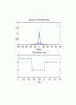
dem=real(ifft(D))*fs; %Demodulate Signal
clf
subplot(2,1,1) %주파수 축에서의 복조 시그널
plot(f,fftshift(abs(D)))
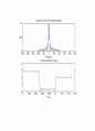
title(\'Spectrum of the Demodulated Signal\')
xlabel(\'Frequency\')
subplot(2,1,2) %시간 축에서의 복조 시그널
plot(t,dem(1:length(t)))
title(\'The Demodulator Output\')
xlabel(\'Time\')
2. [SSB-AM & VSB-AM]
2.1.1 Plot the Hilbert transform of the message signal and the modulated signal u3(t). Also plot the spectrum of the modulated signal u3(t) and compare with the spectrum of the DSB-SC AM modulated signal u1(t).
echo on
t0=0.15;
ts=0.001; %샘플 시간
fc=250; %Frequency
fs=1/ts; %Sample Frequency
df=0.25; %Desired Frequency
t=[0:ts:t0]; %time vector
%message signal
%sample의 0부터 0.05까지 1, 0.51부터 0.10까지 -2, 그 뒤로 0값을 갖는 벡터
m=[ones(1,t0/(3*ts)+1),-2*ones(1,t0/(3*ts)),zeros(1,t0/(3*ts))];
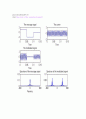
u=m.*cos(2*pi*fc.*t)+imag(hilbert(m)).*sin(2*pi*fc.*t); %LSSB SIGNAL
f=[0:df1:df1*(length(u)-1)]-fs/2; %Frequency Vector
[U,u,df1]=fftseq(u,ts,df);
U=U/fs;
f=[0:df1:df1*(length(u)-1)]-fs/2;
clf
subplot(2,1,1)
plot(t,u(1:length(t)))
xlabel(\'Time\')
title(\'The LSSB-AM modulated signal\')
subplot(2,1,2)
plot(f,abs(fftshift(U)))
xlabel(\'Frequency\')
title(\'Spectrum of the LSSB-AM modulated signal\')
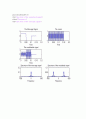
2.1.3 Demodulate the modulated signal u3(t) and recover m(t). Plot the results in the time and frequency domains.
echo on
t0=0.15;
ts=0.001; %샘플 시간
fc=250; %Frequency
fs=1/ts; %Sample Frequency
df=0.25; %Desired Frequency
t=[0:ts:t0]; %time vector
%message signal
%sample의 0부터 0.05까지 1, 0.51부터 0.10까지 -2, 그 뒤로 0값을 갖는 벡터
m=[ones(1,t0/(3*ts)+1),-2*ones(1,t0/(3*ts)),zeros(1,t0/(3*ts))];
u=m.*cos(2*pi*fc.*t)+imag(hilbert(m)).*sin(2*pi*fc.*t); %LSSB SIGNAL
f=[0:df1:df1*(length(u)-1)]-fs/2; %Frequency Vector
c=cos(2*pi*fc.*t) %Demodulator ocilator signal
y=(u.*c); %Demodulation
[Y,y,df1]=fftseq(y,ts,df); %Fourier Transform
Y=Y/fs; %Sample 수 만큼 나눠준다
n_cut=floor(200/df1); %filter design frequency 200에서 짤라준다
f=[0:df1:df1*(length(y)-1)]-fs/2; %Frequency vector
F=zeros(size(f)); %filter vector
F(1:n_cut)=2*ones(1,n_cut);
F(length(f)-n_cut+1:length(f))=2*ones(1,n_cut);
D=F.*Y; %filter 통과
dem=real(ifft(D))*fs; %Demodulate Signal
clf
subplot(2,1,1) %주파수 축에서의 복조 시그널
plot(f,fftshift(abs(D)))
title(\'Spectrum of the Demodulated Signal\')
xlabel(\'Frequency\')
subplot(2,1,2) %시간 축에서의 복조 시그널
plot(t,dem(1:length(t)))
title(\'The Demodulator Output\')
xlabel(\'Time\')
a=0.85; %Modulation index
fs = 1/ts; %Sample Frequency
t=[0:ts:t0]; %Time Vector
df=0.25; %Desired Frequency
%message signal
%sample의 0부터 0.05까지 1, 0.51부터 0.10까지 -2, 그 뒤로 0값을 갖는 벡터
m=[ones(1,t0/(3*ts)+1),-2*ones(1,t0/(3*ts)), zeros(1,t0/(3*ts))];
c=cos(2*pi*fc.*t); %캐리어 시그널
m_n=m/max(abs(m)); %Normalizing
u=(1+a*m_n).*c; %modulating
y=(u.*c)*2-1; %Demodulation
[Y,y,df1]=fftseq(y,ts,df); %Fourier Transform
Y=Y/fs; %Sample 수 만큼 나눠준다
n_cut=floor(200/df1); %filter design frequency 200에서 짤라준다
f=[0:df1:df1*(length(y)-1)]-fs/2; %Frequency vector
F=zeros(size(f)); %filter vector
F(1:n_cut)=2*ones(1,n_cut);
F(length(f)-n_cut+1:length(f))=2*ones(1,n_cut);
D=F.*Y; %filter 통과
dem=real(ifft(D))*fs; %Demodulate Signal
clf
subplot(2,1,1) %주파수 축에서의 복조 시그널
plot(f,fftshift(abs(D)))
title(\'Spectrum of the Demodulated Signal\')
xlabel(\'Frequency\')
subplot(2,1,2) %시간 축에서의 복조 시그널
plot(t,dem(1:length(t)))
title(\'The Demodulator Output\')
xlabel(\'Time\')
2. [SSB-AM & VSB-AM]
2.1.1 Plot the Hilbert transform of the message signal and the modulated signal u3(t). Also plot the spectrum of the modulated signal u3(t) and compare with the spectrum of the DSB-SC AM modulated signal u1(t).
echo on
t0=0.15;
ts=0.001; %샘플 시간
fc=250; %Frequency
fs=1/ts; %Sample Frequency
df=0.25; %Desired Frequency
t=[0:ts:t0]; %time vector
%message signal
%sample의 0부터 0.05까지 1, 0.51부터 0.10까지 -2, 그 뒤로 0값을 갖는 벡터
m=[ones(1,t0/(3*ts)+1),-2*ones(1,t0/(3*ts)),zeros(1,t0/(3*ts))];
u=m.*cos(2*pi*fc.*t)+imag(hilbert(m)).*sin(2*pi*fc.*t); %LSSB SIGNAL
f=[0:df1:df1*(length(u)-1)]-fs/2; %Frequency Vector
[U,u,df1]=fftseq(u,ts,df);
U=U/fs;
f=[0:df1:df1*(length(u)-1)]-fs/2;
clf
subplot(2,1,1)
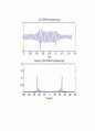
plot(t,u(1:length(t)))
xlabel(\'Time\')
title(\'The LSSB-AM modulated signal\')
subplot(2,1,2)
plot(f,abs(fftshift(U)))
xlabel(\'Frequency\')
title(\'Spectrum of the LSSB-AM modulated signal\')
2.1.3 Demodulate the modulated signal u3(t) and recover m(t). Plot the results in the time and frequency domains.
echo on
t0=0.15;
ts=0.001; %샘플 시간
fc=250; %Frequency
fs=1/ts; %Sample Frequency
df=0.25; %Desired Frequency
t=[0:ts:t0]; %time vector
%message signal
%sample의 0부터 0.05까지 1, 0.51부터 0.10까지 -2, 그 뒤로 0값을 갖는 벡터
m=[ones(1,t0/(3*ts)+1),-2*ones(1,t0/(3*ts)),zeros(1,t0/(3*ts))];
u=m.*cos(2*pi*fc.*t)+imag(hilbert(m)).*sin(2*pi*fc.*t); %LSSB SIGNAL
f=[0:df1:df1*(length(u)-1)]-fs/2; %Frequency Vector
c=cos(2*pi*fc.*t) %Demodulator ocilator signal
y=(u.*c); %Demodulation
[Y,y,df1]=fftseq(y,ts,df); %Fourier Transform
Y=Y/fs; %Sample 수 만큼 나눠준다
n_cut=floor(200/df1); %filter design frequency 200에서 짤라준다
f=[0:df1:df1*(length(y)-1)]-fs/2; %Frequency vector
F=zeros(size(f)); %filter vector
F(1:n_cut)=2*ones(1,n_cut);
F(length(f)-n_cut+1:length(f))=2*ones(1,n_cut);
D=F.*Y; %filter 통과
dem=real(ifft(D))*fs; %Demodulate Signal
clf
subplot(2,1,1) %주파수 축에서의 복조 시그널
plot(f,fftshift(abs(D)))
title(\'Spectrum of the Demodulated Signal\')
xlabel(\'Frequency\')
subplot(2,1,2) %시간 축에서의 복조 시그널
plot(t,dem(1:length(t)))
title(\'The Demodulator Output\')
xlabel(\'Time\')
추천자료
 IT 기술 동향과 전망 및 관련 연구 사례
 RF를 이용한 장애물 피하는 모형자동차
- IT839 - 21c 경제발전 핵심프로젝트
- 현 CRM의 문제점과 앞으로의 개선방향
- [정보화교육]사이버를 활용한 교육 사례 및 활성화 방향
- 와이브로 창업에 관한 프로젝트(양재욱)
- Visual C++을 이용한 CRC구현
- 에듀넷활용학습의 필요성과 장점, 에듀넷활용학습을 통한 협동학습과 멀티미디어학습, 에듀넷...
- [방송통신대]로잘린드 프랭클린과 DNA의 분석 및 서평
- 대구지역 전통산업과 첨단산업의 국제화전략의 비교
 레지오 에밀리아 접근법의 이해와 현장적용위한 방안
- 레지오 에밀리아 접근법의 이해와 현재교육현장에서 적용방안을 논하시오
- 한국방송통신대학교 3학년 1학기 과제. 교육공학. 공통
- 자바 학기말과제, 치킨집 포스기 프로그램입니다.(설치, 실행방법 첨부)
- 가격2,000원
- 페이지수13페이지
- 등록일2006.06.07
- 저작시기2006.6
- 파일형식한글(hwp)
- 자료번호#353725

본 자료는 최근 2주간 다운받은 회원이 없습니다.


소개글