지연상관된 광역규모 예측인자를 이용한 한반도 지역 강수량의 계절 예측

소개글

지연상관된 광역규모 예측인자를 이용한 한반도 지역 강수량의 계절 예측에 대한 보고서 자료입니다.

목차

1. 서론

2. 자료 및 방법

3. 분석결과

4. 결론

5. 참고문헌

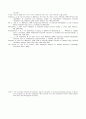
본문내용

2nd
SLP of June
40N,0
0.57
SST of April
57N,162E
-0.53
SLP of January
32.5S,160E
-0.51
850mb GPH of August
35N,17.5W
0.56
3th
SST of May
23S,158W
-0.52
SLP of December
50N,85W
0.60
850mb GPH of April
47.5N,45E
0.49
SST of March
45S,78E
-0.54
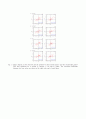
Fig. 1 Scatter diagram of the observed and the predicted of the first(left panels) and the second(right panels) EOF time coefficient for a) spring, b) summer, c) fall and d) winter. The correlation coefficients between two time series are shown in the right lower part of each figure.
Fig. 2 Time series of the observed (solid line) and the predicted (dashed line) for a) spring, b) summer, c) fall and d) winter. The prediction was obtained from super ensemble.
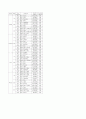
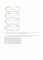
Table 2. The hit rate of categorical prediction for the three classes such as above normal (W), near normal (N) and below normal (D). Obs and Fct indicate observation and prediction, respectively.
Obs
D
N
W
season Fct
D
N
W
D
N
W
D
N
W
Spring
0.55
0.41
0.04
0.21
0.57
0.22
0.05
0.24
0.71
Summer
0.51
0.42
0.07
0.13
0.63
0.24
0.03
0.55
0.42
Fall
0.52
0.43
0.04
0.23
0.52
0.24
0.02
0.25
0.73
Winter
0.50
0.48
0.02
0.21
0.59
0.20
0.03
0.23
0.74
mean
0.52
0.44
0.04
0.20
0.58
0.23
0.03
0.32
0.65

키워드

지연상관,   광역,   예측,   인자,   한바도,   지역,   강수,   계절