MATLAB 사용 방법과 AM, FM,DS-SS 파형관찰 및 소스코드

목차

1 .소 개
1. 1 Communication Theory pp. 11.
1. 2 MATLAB pp. 4

2 .A M
2. 1 AM pp. 82.
2. 2 DSB - SC pp.11
2. 3 VSB pp.14
2. 4 SSB pp.17

3 .F M
3. 1 FM pp.20

4 .DS - SS pp.27

5 .Filter designpp.29

6 .MATLAB source code pp.37

7 .Conclusion pp.45

본문내용

gth(t)-1
int_mt(i+1)=int_mt(i)+mt(i)*Ts;
end
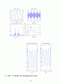
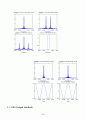
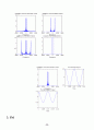
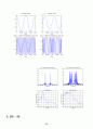
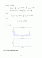
figure(1)
subplot(221)
plot(t,mt);
title('Message signal')
xlabel('Time (sec)')
subplot(222)
plot(t,int_mt);
title('Integral of m(t)')
xlabel('Time (sec)')
kf = 10;
St = cos(2*pi*fc*t + 2*pi*kf*int_mt);
subplot(223)
plot(t,St)
title('The modulated signal S(t) when Beta << 1')
xlabel('Time (sec)')
kf = 500;
St = cos(2*pi*fc*t + 2*pi*kf*int_mt);
subplot(224)
plot(t,St)
title('The modulated signal S(t) when Beta > 1')
xlabel('Time (sec)')
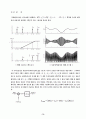
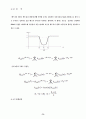
figure(2)
kf = 10;
St = cos(2*pi*fc*t + 2*pi*kf*int_mt);
N = 8000;
F = (-N/2:N/2-1)*fs/N;
S = abs(fft(St,N))/(2*80);
S = fftshift(S);
subplot(221)
plot(F,S)
title('Beta<<1, magnitude-spectrum of the modulated signal')
xlabel('Frequency (Hz)')
kf = 500;
St = cos(2*pi*fc*t + 2*pi*kf*int_mt);
N = 8000;
F = (-N/2:N/2-1)*fs/N;
S = abs(fft(St,N))/(2*80);
S = fftshift(S);
subplot(222)
plot(F,S)
title('Beta>1, magnitude-spectrum of the modulated signal')
xlabel('Frequency (Hz)')
kf = 10;
St = cos(2*pi*fc*t + 2*pi*kf*int_mt);
subplot(223)
psd(St,[],1000)
title('PSD of S(t) when Beta << 1')
kf = 500;
St = cos(2*pi*fc*t + 2*pi*kf*int_mt);
subplot(224)
psd(St,[],1000)
title('PSD of S(t) when Beta > 1')
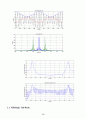
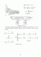
6. 7 Low-Pass filter
clear all
close all
N = 64;
fc = 0.3;
k = 1;
t = ([0:N-1]-(N-1)/2);
f = (1/N)*[-N/2:N/2-1];
h_lpf = k*sin(2*pi*fc*t)./(pi*t);
if rem(N,2) == 0
else
h_lpf((N+1)/2)=2*fc;
end
subplot(211)
plot(t,h_lpf)
xlabel('Time (sec)')
ylabel('h_lpf')
title('Low-Pass filter impulse response')
LPF=fftshift(abs(fft(h_lpf)));
subplot(212)
plot(f,LPF)
xlabel('Frequency (Hz)')
ylabel('Amplitude')
title('Low-Pass filter frequency response')
6. 8 High-Pass filter
clear all
close all
N = 64;
fc = 0.3;
k = 1;
t = ([0:N-1]-(N-1)/2);
f = (1/N)*[-N/2:N/2-1];
h_hpf = (-1).^t*k.*sin(2*pi*(0.5-fc)*t)./(pi*t);
if rem(N,2) == 0
else
h_hpf((N+1)/2)=2*(0.5-fc);
end
subplot(211)
plot(t,h_hpf)
xlabel('Time (sec)')
ylabel('h_hpf')
title('High-Pass filter impulse response')
HPF=fftshift(abs(fft(h_hpf)));
subplot(212)
plot(f,HPF)
xlabel('Frequency (Hz)')
ylabel('Amplitude')
title('High-Pass filter frequency response')
6. 9 Band-Pass filter
clear all
close all
N = 64;
fu = 0.3;
fl = 0.2;
k = 1;
f = (1/N)*[-N/2:N/2-1];
l = find( ((f>=fl)&(f<=fu))|((f>=-fu)&(f<=-fl)));
BPF = zeros(1,N);
BPF(l) = ones(1,length(l))
h_bpf=abs(ifft(BPF));
subplot(211)
plot(h_bpf)
xlabel('Time (sec)')
ylabel('h_bpf')
title('Band-Pass filter impulse response')
subplot(212)
plot(f,BPF)
xlabel('Frequency (Hz)')
ylabel('Amplitude')
title('Band-Pass filter frequency response')
6. 10 Band-stop filter
clear all
close all
N = 64;
fu = 0.3;
fl = 0.2;
k = 1;
f = (1/N)*[-N/2:N/2-1];
l = find( ((f>=fl)&(f<=fu))|((f>=-fu)&(f<=-fl)));
BPF = zeros(1,N);
BPF(l) = ones(1,length(l))
BSF = k*(1-BPF);
h_bsf=abs(ifft(BSF));
subplot(211)
plot(h_bsf)
xlabel('Time (sec)')
ylabel('h_bpf')
title('Band-stop filter impulse response')
subplot(212)
plot(f,BSF)
xlabel('Frequency (Hz)')
ylabel('Amplitude')
title('Band-stop filter frequency response')

키워드

DSB-SC,   AM,   FM,   변복조,   통신이론,   MATLAB,   DS - SS